[TOC]
前言:
Kaggle数据挖掘竞赛:使用随机森林预测泰坦尼克号生存情况
数据来源kaggle
1 数据预处理 1.1 读入数据 1 2 3 4 import pandas as pddata_train = pd.read_csv(r'train.csv' ) data_test = pd.read_csv(r'test.csv' ) data_train.head()
PassengerId
Survived
Pclass
Name
Sex
Age
SibSp
Parch
Ticket
Fare
Cabin
Embarked
0
1
0
3
Braund, Mr. Owen Harris
male
22.0
1
0
A/5 21171
7.2500
NaN
S
1
2
1
1
Cumings, Mrs. John Bradley (Florence Briggs Th...
female
38.0
1
0
PC 17599
71.2833
C85
C
2
3
1
3
Heikkinen, Miss. Laina
female
26.0
0
0
STON/O2. 3101282
7.9250
NaN
S
3
4
1
1
Futrelle, Mrs. Jacques Heath (Lily May Peel)
female
35.0
1
0
113803
53.1000
C123
S
4
5
0
3
Allen, Mr. William Henry
male
35.0
0
0
373450
8.0500
NaN
S
1.2 训练集与数据集
PassengerId
Pclass
Name
Sex
Age
SibSp
Parch
Ticket
Fare
Cabin
Embarked
0
892
3
Kelly, Mr. James
male
34.5
0
0
330911
7.8292
NaN
Q
1
893
3
Wilkes, Mrs. James (Ellen Needs)
female
47.0
1
0
363272
7.0000
NaN
S
2
894
2
Myles, Mr. Thomas Francis
male
62.0
0
0
240276
9.6875
NaN
Q
3
895
3
Wirz, Mr. Albert
male
27.0
0
0
315154
8.6625
NaN
S
4
896
3
Hirvonen, Mrs. Alexander (Helga E Lindqvist)
female
22.0
1
1
3101298
12.2875
NaN
S
1.2.1 查看数据完整性 <class 'pandas.core.frame.DataFrame'>
RangeIndex: 891 entries, 0 to 890
Data columns (total 12 columns):
PassengerId 891 non-null int64
Survived 891 non-null int64
Pclass 891 non-null int64
Name 891 non-null object
Sex 891 non-null object
Age 714 non-null float64
SibSp 891 non-null int64
Parch 891 non-null int64
Ticket 891 non-null object
Fare 891 non-null float64
Cabin 204 non-null object
Embarked 889 non-null object
dtypes: float64(2), int64(5), object(5)
memory usage: 83.7+ KB总共有891组数据,其中age是714条,Cabin是204条,共计12个变量
乘客ID,存活情况,船票级别,乘客姓名,性别,年龄,船上的兄弟姐妹以及配偶的人数,船上的父母以及子女的人数,船票编号,船票费用,所在船舱,登船的港口
1.2.2 查看训练数据描述信息
PassengerId
Survived
Pclass
Age
SibSp
Parch
Fare
count
891.000000
891.000000
891.000000
714.000000
891.000000
891.000000
891.000000
mean
446.000000
0.383838
2.308642
29.699118
0.523008
0.381594
32.204208
std
257.353842
0.486592
0.836071
14.526497
1.102743
0.806057
49.693429
min
1.000000
0.000000
1.000000
0.420000
0.000000
0.000000
0.000000
25%
223.500000
0.000000
2.000000
20.125000
0.000000
0.000000
7.910400
50%
446.000000
0.000000
3.000000
28.000000
0.000000
0.000000
14.454200
75%
668.500000
1.000000
3.000000
38.000000
1.000000
0.000000
31.000000
max
891.000000
1.000000
3.000000
80.000000
8.000000
6.000000
512.329200
mean代表各项的均值,获救率为0.383838
1.3.1 年龄数据简化分组 1 2 3 4 5 6 7 8 9 10 11 12 def simplify_ages (df) : df.Age = df.Age.fillna(-0.5 ) bins = (-1 , 0 , 5 , 12 , 18 , 25 , 35 , 60 , 120 ) group_names = ['Unknown' , 'Baby' , 'Child' , 'Teenager' , 'Student' , 'Young Adult' , 'Adult' , 'Senior' ] catagories = pd.cut(df.Age,bins,labels=group_names) df.Age = catagories return df
简化Cabin,就是取字母
1 2 3 4 def simplify_cabin (df) : df.Cabin = df.Cabin.fillna('N' ) df.Cabin = df.Cabin.apply(lambda x:x[0 ]) return df
简化工资,也就是分组
1 2 3 4 5 6 7 def simplify_fare (df) : df.Fare = df.Fare.fillna(-0.5 ) bins = (-1 , 0 , 8 , 15 , 31 , 1000 ) group_names = ['Unknown' , '1_quartile' , '2_quartile' , '3_quartile' , '4_quartile' ] catagories = pd.cut(df.Fare,bins,labels=group_names) df.Fare = catagories return df
删除无用信息
1 2 def simplify_drop (df) : return df.drop(['Name' ,'Ticket' ,'Embarked' ],axis=1 )
整合一遍,凑成新表
1 2 3 4 5 6 def transform_features (df) : df = simplify_ages(df) df = simplify_cabin(df) df = simplify_fare(df) df = simplify_drop(df) return df
执行读取新表
1 2 3 4 5 data_train = pd.read_csv(r'train.csv' ) data_train = transform_features(data_train) data_test = transform_features(data_test) data_train.head()
PassengerId
Survived
Pclass
Sex
Age
SibSp
Parch
Fare
Cabin
0
1
0
3
male
Student
1
0
1_quartile
N
1
2
1
1
female
Adult
1
0
4_quartile
C
2
3
1
3
female
Young Adult
0
0
1_quartile
N
3
4
1
1
female
Young Adult
1
0
4_quartile
C
4
5
0
3
male
Young Adult
0
0
2_quartile
N
Survived
Pclass
Sex
Age
SibSp
Parch
Ticket
Fare
Embarked
0
0
3
male
22.0
1
0
A/5 21171
7.2500
S
1
1
1
female
38.0
1
0
PC 17599
71.2833
C
2
1
3
female
26.0
0
0
STON/O2. 3101282
7.9250
S
3
1
1
female
35.0
1
0
113803
53.1000
S
4
0
3
male
35.0
0
0
373450
8.0500
S
...
...
...
...
...
...
...
...
...
...
195
1
1
female
58.0
0
0
PC 17569
146.5208
C
196
0
3
male
NaN
0
0
368703
7.7500
Q
197
0
3
male
42.0
0
1
4579
8.4042
S
198
1
3
female
NaN
0
0
370370
7.7500
Q
199
0
2
female
24.0
0
0
248747
13.0000
S
200 rows × 9 columns
选取我们需要的那几个列作为输入, 对于票价和姓名我就舍弃了,姓名没什么用
1 2 3 cols = ['PassengerId' ,'Survived' ,'Pclass' ,'Sex' ,'Age' ,'SibSp' ,'Parch' ,'Fare' ,'Embarked' ] data_tr=data_train[cols].copy() data_tr.head()
PassengerId
Survived
Pclass
Sex
Age
SibSp
Parch
Fare
Embarked
0
1
0
3
male
22.0
1
0
7.2500
S
1
2
1
1
female
38.0
1
0
71.2833
C
2
3
1
3
female
26.0
0
0
7.9250
S
3
4
1
1
female
35.0
1
0
53.1000
S
4
5
0
3
male
35.0
0
0
8.0500
S
1 2 3 cols = ['PassengerId' ,'Pclass' ,'Sex' ,'Age' ,'SibSp' ,'Parch' ,'Fare' ,'Embarked' ] data_te=data_test[cols].copy() data_te.head()
PassengerId
Pclass
Sex
Age
SibSp
Parch
Fare
Embarked
0
892
3
male
34.5
0
0
7.8292
Q
1
893
3
female
47.0
1
0
7.0000
S
2
894
2
male
62.0
0
0
9.6875
Q
3
895
3
male
27.0
0
0
8.6625
S
4
896
3
female
22.0
1
1
12.2875
S
1 2 data_tr.isnull().sum() data_te.isnull().sum()
PassengerId 0
Pclass 0
Sex 0
Age 86
SibSp 0
Parch 0
Fare 1
Embarked 0
dtype: int64填充数据,,,,,,
1 2 3 4 age_mean = data_tr['Age' ].mean() data_tr['Age' ] = data_tr['Age' ].fillna(age_mean) data_tr['Embarked' ] = data_tr['Embarked' ].fillna('S' ) data_tr.isnull().sum()
PassengerId 0
Survived 0
Pclass 0
Sex 0
Age 0
SibSp 0
Parch 0
Fare 0
Embarked 0
dtype: int64
PassengerId
Survived
Pclass
Sex
Age
SibSp
Parch
Fare
Embarked
0
1
0
3
male
22.0
1
0
7.2500
S
1
2
1
1
female
38.0
1
0
71.2833
C
2
3
1
3
female
26.0
0
0
7.9250
S
3
4
1
1
female
35.0
1
0
53.1000
S
4
5
0
3
male
35.0
0
0
8.0500
S
用数组特征化编码年龄和S C Q等等,,因为随机森林的输入需要数值,字符不行
1 2 3 4 5 6 7 8 9 10 age_mean = data_te['Age' ].mean() data_te['Age' ] = data_te['Age' ].fillna(age_mean) age_mean = data_te['Fare' ].mean() data_te['Fare' ] = data_te['Fare' ].fillna(age_mean) data_te['Sex' ]= data_te['Sex' ].map({'female' :0 , 'male' : 1 }).astype(int) data_te['Embarked' ]= data_te['Embarked' ].map({'S' :0 , 'C' : 1 ,'Q' :2 }).astype(int) data_te.head()
PassengerId
Pclass
Sex
Age
SibSp
Parch
Fare
Embarked
0
892
3
1
34.5
0
0
7.8292
2
1
893
3
0
47.0
1
0
7.0000
0
2
894
2
1
62.0
0
0
9.6875
2
3
895
3
1
27.0
0
0
8.6625
0
4
896
3
0
22.0
1
1
12.2875
0
1 2 3 4 data_tr['Sex' ]= data_tr['Sex' ].map({'female' :0 , 'male' : 1 }).astype(int) data_tr['Embarked' ]= data_tr['Embarked' ].map({'S' :0 , 'C' : 1 ,'Q' :2 }).astype(int) data_tr.head()
PassengerId
Survived
Pclass
Sex
Age
SibSp
Parch
Fare
Embarked
0
1
0
3
1
22.0
1
0
7.2500
0
1
2
1
1
0
38.0
1
0
71.2833
1
2
3
1
3
0
26.0
0
0
7.9250
0
3
4
1
1
0
35.0
1
0
53.1000
0
4
5
0
3
1
35.0
0
0
8.0500
0
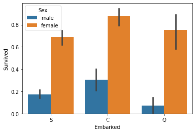
2 数据可视化 2.1 年龄和生存率之间的关系 1 sns.barplot(x='Embarked' ,y='Survived' ,hue='Sex' ,data=data_train)
<matplotlib.axes._subplots.AxesSubplot at 0x7fee5875e3c8>
female的获救率大于 male,(应该是男士都比较绅士吧,即使面对死亡,也希望将最后的机会留给女生,,电影感悟)
获救率 C 男性女性都是最高,Q时男性最低,S 时 女性最低
男性的获救率低于女性的三分之一
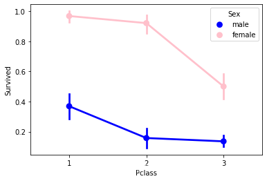
2.2 所做的位置和生存率之间的关系 1 2 sns.pointplot(x='Pclass' ,y='Survived' ,hue='Sex' ,data=data_train,palette={'male' :'blue' ,'female' :'pink' }, marker=['*' ,"o" ],linestyle=['-' ,'--' ])
<matplotlib.axes._subplots.AxesSubplot at 0x7fee586f70b8>
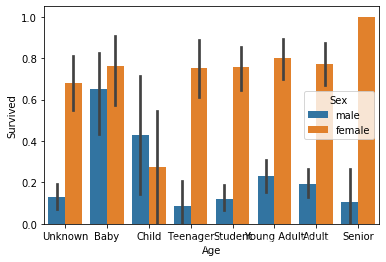
2.3 生存率与年龄的关系 1 sns.barplot(x = 'Age' ,y = 'Survived' ,hue='Sex' ,data = data_train)
<matplotlib.axes._subplots.AxesSubplot at 0x7fee587238d0>
男性大于女性
student的生存率最低,bady的生存率最高
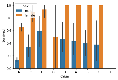
1 sns.barplot(x = 'Cabin' ,y = 'Survived' ,hue='Sex' ,data = data_train)
<matplotlib.axes._subplots.AxesSubplot at 0x7fee585b0748>
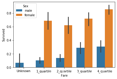
1 sns.barplot(x = 'Fare' ,y = 'Survived' ,hue='Sex' ,data = data_train)
<matplotlib.axes._subplots.AxesSubplot at 0x7fee5852b390>
3 建立模型 3.1 随机森林 1 2 3 4 5 6 7 8 9 10 11 12 13 14 15 16 17 18 19 20 21 22 23 24 25 26 27 28 29 30 31 32 33 34 35 36 from sklearn.model_selection import train_test_splitX_all = data_tr.drop(['PassengerId' ,'Survived' ],axis=1 ) y_all = data_tr['Survived' ] p = 0.2 X_train,X_test, y_train, y_test = train_test_split(X_all,y_all,test_size=p, random_state=23 ) from sklearn.ensemble import RandomForestClassifierfrom sklearn.metrics import make_scorer, accuracy_scorefrom sklearn.model_selection import GridSearchCVclf = RandomForestClassifier() parameters = {'n_estimators' : [4 , 6 , 9 ], 'max_features' : ['log2' , 'sqrt' ,'auto' ], 'criterion' : ['entropy' , 'gini' ], 'max_depth' : [2 , 3 , 5 , 10 ], 'min_samples_split' : [2 , 3 , 5 ], 'min_samples_leaf' : [1 ,5 ,8 ] } acc_scorer = make_scorer(accuracy_score) grid_obj = GridSearchCV(clf,parameters,scoring=acc_scorer) grid_obj = grid_obj.fit(X_train,y_train) clf = grid_obj.best_estimator_ clf.fit(X_train,y_train)
/home/wvdon/anaconda3/envs/weidong/lib/python3.7/site-packages/sklearn/model_selection/_split.py:1978: FutureWarning: The default value of cv will change from 3 to 5 in version 0.22. Specify it explicitly to silence this warning.
warnings.warn(CV_WARNING, FutureWarning)
/home/wvdon/anaconda3/envs/weidong/lib/python3.7/site-packages/sklearn/model_selection/_search.py:814: DeprecationWarning: The default of the `iid` parameter will change from True to False in version 0.22 and will be removed in 0.24. This will change numeric results when test-set sizes are unequal.
DeprecationWarning)
RandomForestClassifier(bootstrap=True, class_weight=None, criterion='entropy',
max_depth=5, max_features='sqrt', max_leaf_nodes=None,
min_impurity_decrease=0.0, min_impurity_split=None,
min_samples_leaf=1, min_samples_split=3,
min_weight_fraction_leaf=0.0, n_estimators=4,
n_jobs=None, oob_score=False, random_state=None,
verbose=0, warm_start=False)3.2 预测 1 2 3 predictions = clf.predict(X_test) print(accuracy_score(y_test,predictions)) data_tr
0.8268156424581006
PassengerId
Survived
Pclass
Sex
Age
SibSp
Parch
Fare
Embarked
0
1
0
3
1
22.000000
1
0
7.2500
0
1
2
1
1
0
38.000000
1
0
71.2833
1
2
3
1
3
0
26.000000
0
0
7.9250
0
3
4
1
1
0
35.000000
1
0
53.1000
0
4
5
0
3
1
35.000000
0
0
8.0500
0
...
...
...
...
...
...
...
...
...
...
886
887
0
2
1
27.000000
0
0
13.0000
0
887
888
1
1
0
19.000000
0
0
30.0000
0
888
889
0
3
0
29.699118
1
2
23.4500
0
889
890
1
1
1
26.000000
0
0
30.0000
1
890
891
0
3
1
32.000000
0
0
7.7500
2
891 rows × 9 columns
3.3 预测test文件 1 2 3 4 predictions = clf.predict(data_te.drop('PassengerId' ,axis=1 )) output = pd.DataFrame({'Passengers' :data_te['PassengerId' ],'Survived' :predictions}) output.to_csv(r'test1.csv' ) output.head()
Passengers
Survived
0
892
0
1
893
0
2
894
0
3
895
0
4
896
0
3.4 提交到kaggle官网 结果是 0.77990