scikit-learn:
- 简单高效的数据挖掘和数据分析工具
前言
Getting Started
Fitting and predicting: estimator basics
- estimators 提供一系列封装好的机器学习算法。
- fit :fit到模型数据。
Example:
1 | from sklearn.ensemble import RandomForestClassifier |
Transformers and pre-processors
- ColumnTransformer : 不同特征的转换处理
sklearn.preprocessing 包含了比较多的数据预处理方法(放缩,编码),能在pipeline应用的同时,也是安全的da ta leakage
1 | StandardScaler |
Pipelines: chaining pre-processors and estimators
整合数据预处理与模型评估到一个pipeline上。
1 | from sklearn.preprocessing import StandardScaler |
Model evaluation
预测的数据,有时候不能很好的拟合到test数据,可能是泛化能力不好,也有可能是数据的split导致的train和test两部分数据的差异。可以利用交叉验证,在不同划分的数据上都进行拟合。
1 | from sklearn.datasets import make_regression |
Automatic parameter searches
Scikit-learn 提供了自动超参数的搜索工具。把最好的参数fit到模型上。
1 | from sklearn.datasets import fetch_california_housing |
pre-processing
Data Leakage
Why? :independence between training and testing data.
how to prevent it:Using a pipeline for cross-validation and searching will largely keep you from this common pitfall
数据包
sklearn datasets
提供一些导入,在线下载及本地生成数据集的方法。
sklearn.datasets模块主要提供了一些导入、在线下载及本地生成数据集的方法,可以通过dir或help命令查看,我们会发现主要有三种形式:load_
、fetch_ 及make_ 的方法
train_test_split
1 | from sklearn.model_selection import train_test_splitX_train,X_test,y_train,y_test = train_test_split(X,y,random_state = 2003) |
线性模型
1 | from sklearn import datasets, linear_model # 引用 sklearn库,主要为了使用其中的线性回归模块 |
KNN
模型的泛化能力:它在新的环境中的适应能力
1 | from sklearn.neighbors import KNeighborsClassifierclf = KNeighborsClassifier(n_neighbors=3)clf.fit(X_train,y_train)correct = np.count_nonzero((clf.predict(X_test)==y_test==True)print("auc is:%3.f"%(corrrect/len(X_test)) |
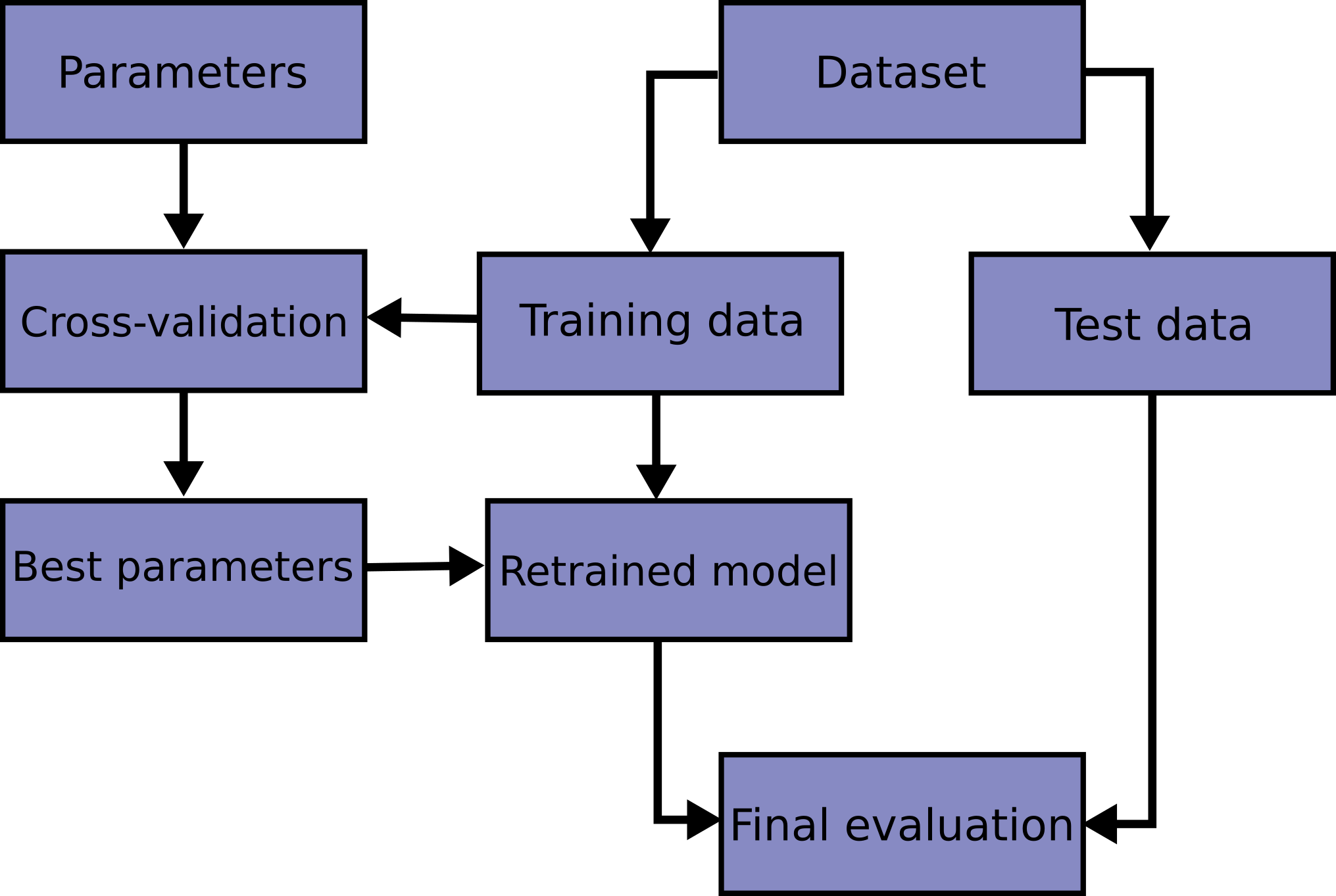
交叉验证
把数据集分为训练集和测试集
常用的交叉验证技术叫做K折交叉验证(K-fold Cross Validation)。 我们先把训练数据再分成训练集和验证集,之后使用训练集来训练模型,然后再验证集上评估模型的准确率。举个例子,比如一个模型有个参数叫\alphaα,我们一开始不清楚要选择0.1还是1,所以这时候我们进行了交叉验证:把所有训练集分成K块,依次对每一个\alphaα值评估它的准确率。下面的动画讲述了如何使用K折交叉验证选出最合适的参数值。
leave_one_out交叉验证,也就是每次只把一个样本当做验证数据,剩下的其他数据都当做是训练样本。
1 | form sklearn.model_selection import GirdSearchCVknn = KNeighborsClassifier()clf = GirdSearchCV(knn,parameters,cv=5)clf.fit(x,y) |
- 绝对不能把测试数据用在交叉验证的过程中
特征缩放
目的是为了:消除有些变量变化的影响
1 线性归一化(Min-max normalization)
线性归一化指的是把特征值的范围映射到[0,1]区间
x_new = (x - min())/(max()-min())
2 标准差标准化 (Z-score Normalization)
特征值映射到均值为0,标准差为1的正态分布 x_new = (x-mean(x)/std(x)
mean(x) x 的平均值 std(x) x的标注差
KNN总结:
- knn 是一个及其简单的算法
- 算法比较适合低纬空间
- KNN 在训练过程中实质上不需要做任何事情,所以训练本身不产生任何时间上的消耗。
merry-based instance -based (实际上没有训练学习的过程)
- KNN预测的时候要循环所以的样本数据,复杂度依赖于样本个数,达成KNN应用在大数据的瓶颈。。
结构化数据与非结构化数据
非结构化数据:简单来讲,文本、图片、声音、视频这些都属于非结构化数据,需要做进一步的处理 结构化的数据指的是存放在数据库里的年龄,身高等这种信息
图像
图像来说,此过程相对简单。一般可以通过Python自带的库来读取图片,并把图片数据存放在矩阵(Matrix)或者张量(Tensor)里 - 图片是由像素来构成的,比如256*256或者128*128。两个值分别代表长宽上的像素。这个值越大图片就会越清晰。另外,对于彩色的图片,一个像素点一般由三维数组来构成,分别代表的是R,G,B三种颜色。除了RGB,其实还有其他常用的色彩空间。如果使用RGB来表示每一个像素点,一个大小为128*128像素的图片实际大小为128*128*3,是一个三维张量的形式。
图片特征
颜色特征(color histigram)
SIFT (Scale-invariant feature transfarm)
它是一个局部的特征,它会试图去寻找图片中的拐点这类的关键点,然后再通过一系列的处理最终得到一个SIFT向量
HOG (Histogram of Oriented Grandient)
通过计算和统计图像局部区域的梯度方向直方图来构建特征.由于HOG是在图像的局部方格单元上操作,所以它对图像几何的和光学的形变都能保持很好的不变性
降维
对于一个中小型图片,它的大小一般大于2562563。如果把它转换成向量,其实维度的大小已经几十万了。这会导致消耗非常大的计算资源,所以一般情况下我们都会尝试对图片做一些降维操作。其实特征提取过程我们自然地可以理解为是降维过程。
降维操作会更好地保留图片中重要的信息,同时也帮助过滤掉无用的噪声
PCA(Principal Component Analysis), (常用的降维工具)
它是一种无监督的学习方法,可以把高维的向量映射到低维的空间里。它的核心思路是对数据做线性的变换,然后在空间里选择信息量最大的Top K维度作为新的特征值
matplotlib.pyplot(画图,展示图片)
1 | import matplotlib.pyplot as plt# 读取图片img = plt.imread('')print(img.shape)plt.imshow(im445555555555555g) |
缺失值次5
删除缺失的行 或者缺失的列
填补缺失值:
- 均值,最小值,最大值,特殊值填充 ,中位值
特征编码
把非数值型数据转为数值型
数据独热编码(one-hot encoding) 标签编码
标签编码不能直接作为特征输入到模型中,
因为1,2,3,,,,连续的特征标签,模型是会认为这些类别是有大小关系的。
而独热编码是平行的。
如果我们直接把类别特征看作是具体的数比如0,1,2… 那这时候,数与数之间是有大小关系的,比如2要大于1,1要大于0,而且这些大小相关的信息必然会用到模型当中 但这就跟原来特征的特点产生了矛盾,因为对于深度学习,数据分析来说它们之间并不存在所谓的“大小”,可以理解为平行关系。所以对于这类特征来说,直接用0,1,2.. 的方式来表示是存在问题的,所以结论是不能这么做。
数值型的变量 可以当做特征直接输入,也可以进行离散化操作